Preparing your lesson…正在准备你的课程…正在準備你的課程…Preparando tu lección…Préparation de votre leçon…Deine Lektion wird vorbereitet…Sto preparando la tua lezione…Preparando sua aula…レッスンを準備しています…수업을 준비하고 있어요…Menyediakan pelajaran anda…Menyiapkan pelajaranmu…
Preparing your lesson…正在准备你的课程…正在準備你的課程…Preparando tu lección…Préparation de votre leçon…Deine Lektion wird vorbereitet…Sto preparando la tua lezione…Preparando sua aula…レッスンを準備しています…수업을 준비하고 있어요…Menyediakan pelajaran anda…Menyiapkan pelajaranmu…
We have shown how to use the first and second derivatives of a function to describe the shape of a graph. To graph a function f defined on an unbounded domain, we also need to know the behavior of f as x→±∞. In this section, we define limits at infinity and show how these limits affect the graph of a function. At the end of this section, we outline a strategy for graphing an arbitrary function f.
Limits at Infinity
We begin by examining what it means for a function to have a finite limit at infinity. Then we study the idea of a function with an infinite limit at infinity. Back in Introduction to Functions and Graphs, we looked at vertical asymptotes; in this section we deal with horizontal and oblique asymptotes.
Limits at Infinity and Horizontal Asymptotes
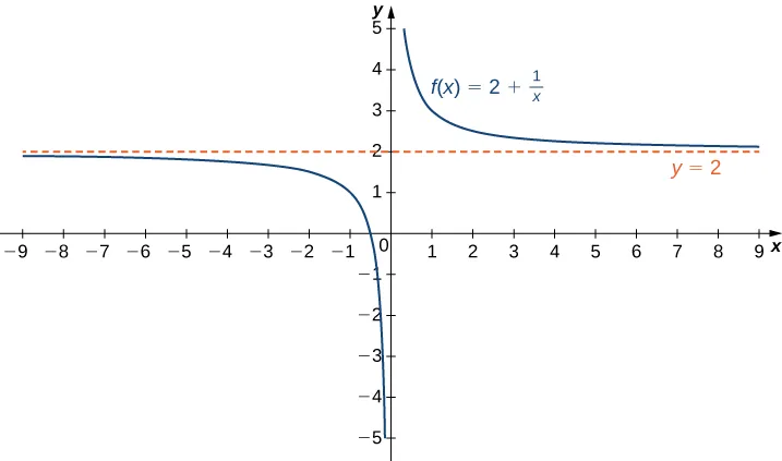
Recall that limx→af(x)=L means f(x) becomes arbitrarily close to L as long as x is sufficiently close to a. We can extend this idea to limits at infinity. For example, consider the function f(x)=2+x1. As can be seen graphically in Figure 4.40 and numerically in Table 4.2, as the values of get larger, the values of approach We say the limit as approaches of is and write Similarly, for as the values get larger, the values of approaches We say the limit as approaches of is and write
Figure 4.40The function approaches the asymptote y=2 as x approaches ±∞.
Table 4.2Values of a function f as x→±∞
x
10
100
1,000
10,000
More generally, for any function f, we say the limit as x→∞ of f(x) is L if f(x) becomes arbitrarily close to L as long as x is sufficiently large. In that case, we write limx→∞f(x)=L. Similarly, we say the limit as of is if becomes arbitrarily close to as long as and is sufficiently large. In that case, we write We now look at the definition of a function having a limit at infinity.
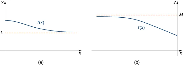
If the values f(x) are getting arbitrarily close to some finite value L as x→∞ or x→-∞, the graph of f approaches the line y=L. In that case, the line y=L is a horizontal asymptote of (Figure 4.41). For example, for the function since the line is a horizontal asymptote of
Figure 4.41(a) As x→∞, the values of f are getting arbitrarily close to L. The line y=L is a horizontal asymptote of f. (b) As x→-∞, the values of are getting arbitrarily close to The line is a horizontal asymptote of
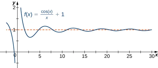
A function cannot cross a vertical asymptote because the graph must approach infinity (or -∞) from at least one direction as x approaches the vertical asymptote. However, a function may cross a horizontal asymptote. In fact, a function may cross a horizontal asymptote an unlimited number of times. For example, the function f(x)=x(cosx)+1 shown in Figure 4.42 intersects the horizontal asymptote an infinite number of times as it oscillates around the asymptote with ever-decreasing amplitude.
Figure 4.42The graph of f(x)=(cosx)/x+1 crosses its horizontal asymptote y=1 an infinite number of times.
The algebraic limit laws and squeeze theorem we introduced in Introduction to Limits also apply to limits at infinity. We illustrate how to use these laws to compute several limits at infinity.
Infinite Limits at Infinity
Sometimes the values of a function f become arbitrarily large as x→∞ (or as x→-∞). In this case, we write limx→∞f(x)=∞ (or limx→-∞f(x)=∞). On the other hand, if the values of are negative but become arbitrarily large in magnitude as (or as we write (or
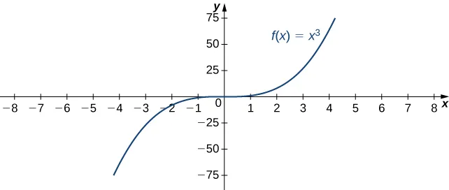
For example, consider the function f(x)=x3. As seen in Table 4.3 and Figure 4.47, as x→∞ the values f(x) become arbitrarily large. Therefore, limx→∞x3=∞. On the other hand, as the values of are negative but become arbitrarily large in magnitude. Consequently,
Table 4.3Values of a power function as x→±∞
x
10
20
50
100
1000
x3
Figure 4.47For this function, the functional values approach infinity as x→±∞.
Formal Definitions
Earlier, we used the terms arbitrarily close, arbitrarily large, and sufficiently large to define limits at infinity informally. Although these terms provide accurate descriptions of limits at infinity, they are not precise mathematically. Here are more formal definitions of limits at infinity. We then look at how to use these definitions to prove results involving limits at infinity.
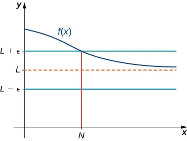
Figure 4.48For a function with a limit at infinity, for all x>N,∣f(x)−L∣<ε.
Earlier in this section, we used graphical evidence in Figure 4.40 and numerical evidence in Table 4.2 to conclude that limx→∞(2+x1)=2. Here we use the formal definition of limit at infinity to prove this result rigorously.
We now turn our attention to a more precise definition for an infinite limit at infinity.
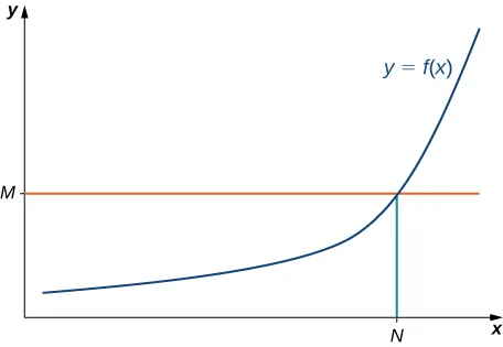
Figure 4.49For a function with an infinite limit at infinity, for all x>N,f(x)>M.
Earlier, we used graphical evidence (Figure 4.47) and numerical evidence (Table 4.3) to conclude that limx→∞x3=∞. Here we use the formal definition of infinite limit at infinity to prove that result.
End Behavior
The behavior of a function as x→±∞ is called the function’s end behavior. At each of the function’s ends, the function could exhibit one of the following types of behavior:
The function f(x) approaches a horizontal asymptote y=L.
The function f(x)→∞ or f(x)→-∞.
The function does not approach a finite limit, nor does it approach ∞ or -∞. In this case, the function may have some oscillatory behavior.
Let’s consider several classes of functions here and look at the different types of end behaviors for these functions.
End Behavior for Polynomial Functions
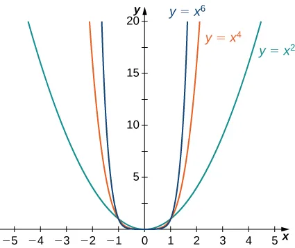
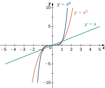
Consider the power function f(x)=xn where n is a positive integer. From Figure 4.50 and Figure 4.51, we see that
x→∞limxn=∞;n=1,2,3,…
and
x→-∞limxn={∞;n=2,4,6,…-∞;n=1,3,5,….
Figure 4.50For power functions with an even exponent of n,limx→∞xn=∞=limx→-∞xn.Figure 4.51For power functions with an odd exponent of n,limx→∞xn=∞ and limx→-∞xn=-∞.
Using these facts, it is not difficult to evaluate limx→∞cxn and limx→-∞cxn, where c is any constant and is a positive integer. If the graph of is a vertical stretch or compression of and therefore
If c=0,y=cxn=0, in which case limx→∞cxn=0=limx→-∞cxn.
We now look at how the limits at infinity for power functions can be used to determine limx→±∞f(x) for any polynomial function f. Consider a polynomial function
f(x)=anxn+an−1xn−1+…+a1x+a0
of degree n≥1 so that an=0. Factoring, we see that
As x→±∞, all the terms inside the parentheses approach zero except the first term. We conclude that
x→±∞limf(x)=x→±∞limanxn.
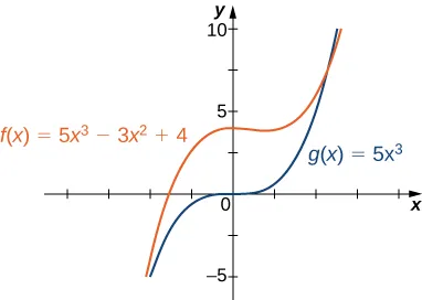
For example, the function f(x)=5x3−3x2+4 behaves like g(x)=5x3 as x→±∞ as shown in Figure 4.52 and Table 4.4.
Figure 4.52The end behavior of a polynomial is determined by the behavior of the term with the largest exponent.
Table 4.4A polynomial’s end behavior is determined by the term with the largest exponent.
x
10
100
1000
f(x)=5x3−3x2+4
End Behavior for Algebraic Functions
The end behavior for rational functions and functions involving radicals is a little more complicated than for polynomials. In Example 4.25, we show that the limits at infinity of a rational function f(x)=q(x)p(x) depend on the relationship between the degree of the numerator and the degree of the denominator. To evaluate the limits at infinity for a rational function, we divide the numerator and denominator by the highest power of x appearing in the denominator. This determines which term in the overall expression dominates the behavior of the function at large values of x.
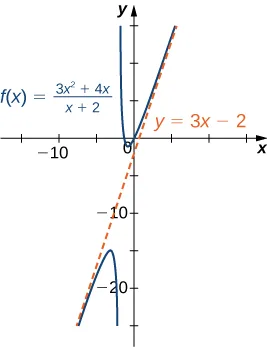
Before proceeding, consider the graph of f(x)=(x+2)(3x2+4x) shown in Figure 4.56. As x→∞ and x→-∞, the graph of appears almost linear. Although is certainly not a linear function, we now investigate why the graph of seems to be approaching a linear function. First, using long division of polynomials, we can write
f(x)=x+23x2+4x=3x−2+x+24.
Since (x+2)4→0 as x→±∞, we conclude that
x→±∞lim(f(x)−(3x−2))=x→±∞limx+24=0.
Therefore, the graph of f approaches the line y=3x−2 as x→±∞. This line is known as an oblique asymptote for f (Figure 4.56).
Figure 4.56The graph of the rational function f(x)=(3x2+4x)/(x+2) approaches the oblique asymptote y=3x−2asx→±∞.
We can summarize the results of Example 4.25 to make the following conclusion regarding end behavior for rational functions. Consider a rational function
If the degree of the numerator is the same as the degree of the denominator (n=m), then f has a horizontal asymptote of y=an/bm as x→±∞.
Determining End Behavior for Transcendental Functions
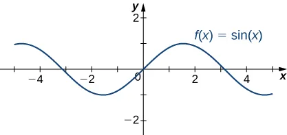
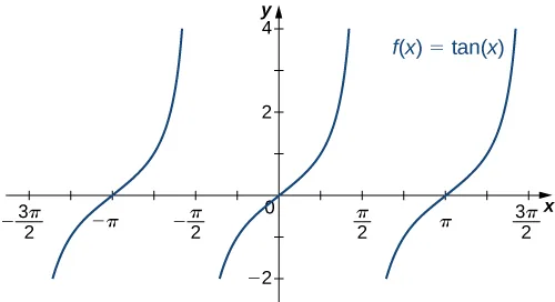
The six basic trigonometric functions are periodic and do not approach a finite limit as x→±∞. For example, sinx oscillates between 1and−1 (Figure 4.58). The tangent function, tan(x), has an infinite number of vertical asymptotes as x→±∞; therefore, it does not approach a finite limit nor does it approach ±∞ as as shown in Figure 4.59.
Figure 4.58The function f(x)=sinx oscillates between 1and−1 as x→±∞Figure 4.59The function f(x)=tanx does not approach a limit and does not approach ±∞ as x→±∞
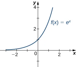
Recall that for any base b>0,b=1, the function y=bx is an exponential function with domain (-∞,∞) and range (0,∞). If is increasing over If is decreasing over For the natural exponential function Therefore, is increasing on and the range is The exponential function approaches as and approaches as as shown in Table 4.5 and Figure 4.60.
Table 4.5End behavior of the natural exponential function
x
−5
−2
0
2
5
ex
Figure 4.60The exponential function approaches zero as x→-∞ and approaches ∞ as x→∞.
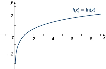
Recall that the natural logarithm function f(x)=ln(x) is the inverse of the natural exponential function y=ex. Therefore, the domain of f(x)=ln(x) is (0,∞) and the range is (-∞,∞). The graph of is the reflection of the graph of about the line Therefore, as and as as shown in Figure 4.61 and Table 4.6.
Table 4.6End behavior of the natural logarithm function
x
0.01
0.1
1
10
100
ln(x)
−4.605
Figure 4.61The natural logarithm function approaches ∞ as x→∞.
Guidelines for Drawing the Graph of a Function
We now have enough analytical tools to draw graphs of a wide variety of algebraic and transcendental functions. Before showing how to graph specific functions, let’s look at a general strategy to use when graphing any function.
Now let’s use this strategy to graph several different functions. We start by graphing a polynomial function.
Key Concepts
The limit of f(x) is L as x→∞ (or as x→-∞) if the values f(x) become arbitrarily close to L as x becomes sufficiently large.
The limit of f(x) is as if becomes arbitrarily large as becomes sufficiently large. The limit of is as if and becomes arbitrarily large as becomes sufficiently large. We can define the limit of as approaches similarly.
x
f(x)
2.
x
∞
f(x)
2
limx→∞f(x)=2.
x<0,
∣x∣
f(x)
2.
x
-∞
f(x)
2
limx→−∞f(x)=2.
2+x1
2.1
2.01
2.001
2.0001
x
−10
−100
−1000
−10,000
2+x1
1.9
1.99
1.999
1.9999
x→-∞
f(x)
L
f(x)
L
x<0
∣x∣
limx→-∞f(x)=L.
If the values of f(x) becomes arbitrarily close to L for x<0 as ∣x∣ becomes sufficiently large, we say that the function f has a limit at negative infinity and write
x→−∞limf(x)=L.
f
f(x)=x1,
limx→∞f(x)=0,
y=0
f(x)=x1.
y=L
horizontal asymptote
f.
f
M.
y=M
f.
y=1
f(x)=5−x22
f(x)=xsinx
f(x)=tan−1(x)
Solution
Using the algebraic limit laws, we have limx→∞(5−x22)=limx→∞5−2(limx→∞x1).(limx→∞x1)=5−2⋅0=5. Similarly, limx→−∞f(x)=5. Therefore, f(x)=5−x22 has a horizontal asymptote of y=5 and f approaches this horizontal asymptote as as shown in the following graph.
Since −1≤sinx≤1 for all x, we have x−1≤xsinx≤x1
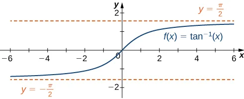
To evaluate limx→∞tan−1(x) and limx→-∞tan−1(x), we first consider the graph of y=tan(x) over the interval as shown in the following graph.
Since
x→(π/2)−limtanx=∞,
it follows that
x→∞limtan−1(x)=2π.
Similarly, since
x→(−π/2)+limtanx=-∞,
it follows that
x→-∞limtan−1(x)=−2π.
As a result, y=2π and y=−2π are horizontal asymptotes of as shown in the following graph.
Figure 4.46This function has two horizontal asymptotes.
f(x)=3+x4,
Hint
limx→±∞1/x=0
Answer
Both limits are 3. The line y=3 is a horizontal asymptote.
f
x→∞
x→-∞),
limx→∞f(x)=-∞
limx→-∞f(x)=-∞).
x→-∞,
f(x)=x3
limx→-∞x3=-∞.
1000
8000
125,000
1,000,000
1,000,000,000
x
−10
−20
−50
−100
−1000
x3
−1000
−8000
−125,000
−1,000,000
−1,000,000,000
if f(x)<0 and ∣f(x)∣ becomes arbitrarily large for x sufficiently large. Similarly, we can define infinite limits as x→-∞.
for all x>N. In that case, we write
x→∞limf(x)=L
(see Figure 4.48).
We say a function f has a limit at negative infinity if there exists a real number L such that for all ε>0, there exists N<0 such that
∣f(x)−L∣<ε
for all x<N. In that case, we write
x→-∞limf(x)=L.
N=ε1.
x>N,
∣2+x1−2∣=∣x1∣=x1<N1=ε.
Hint
Let N=ε1.
Answer
Let ε>0. Let N=ε1. Therefore, for all x>N, we have
∣3−x21−3∣=x21<N21=ε
Therefore, limx→∞(3−1/x2)=3.
f(x)>M
for all x>N (see Figure 4.49).
We say a function has a negative infinite limit at infinity and write
x→∞limf(x)=-∞
if for all M<0, there exists an N>0 such that
f(x)<M
for all x>N.
Similarly we can define limits as x→-∞.
x>N,
x3>N3=(3M)3=M.
Therefore, limx→∞x3=∞.
Answer
Let M>0. Let N=3M. Then, for all x>N, we have
3x2>3N2=3(3M)22=33M=M
n
c>0,
y=cxn
y=xn,
f(x)=2x4
Solution
Since the coefficient of x3 is −5, the graph of f(x)=−5x3 involves a vertical stretch and reflection of the graph of y=x3 about the x-axis. Therefore, limx→∞(−5x3)=-∞ and limx→-∞(−5x3)=∞.
Since the coefficient of x4 is 2, the graph of f(x)=2x4 is a vertical stretch of the graph of y=x4. Therefore, limx→∞2x4=∞ and
Answer
-∞
4704
4,970,004
4,997,000,004
g(x)=5x3
5000
5,000,000
5,000,000,000
x
−10
−100
−1000
f(x)=5x3−3x2+4
−5296
−5,029,996
−5,002,999,996
g(x)=5x3
−5000
−5,000,000
−5,000,000,000
Note:
f(x)=4x3−5x+73x2+2x (Note: The degree of numerator is less than the degree of the denominator.)
f(x)=x+23x2+4x (Note: The degree of numerator is greater than the degree of the denominator.)
Solution
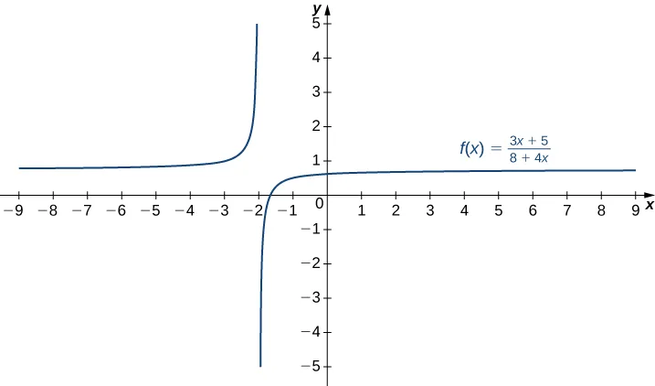
The highest power of x in the denominator is x. Therefore, dividing the numerator and denominator by x and applying the algebraic limit laws, we see that limx→±∞2x+53x−1=limx→±∞2+5/x3−1/x=limx→±∞(2+5/x)limx→±∞(3−1/x)=limx→±∞2+limx→±∞5/xlimx→±∞3−limx→±∞1/x=2+03−0=23. Since limx→±∞f(x)=23, we know that y=23 is a horizontal asymptote for this function as shown in the following graph.
Since the largest power of x appearing in the denominator is x3, divide the numerator and denominator by x3. After doing so and applying algebraic limit laws, we obtain x→±∞lim4x3−5x+73x2+2x=x→±∞lim4−5/x2+7/x33/x+2/x2=4−5(0)+7(0)3(0)+2(0)=0.
Dividing the numerator and denominator by x, we have x→±∞limx+23x2+4x=x→±∞lim1+2/x3x+4.
f(x)=5x2−4x+73x2+2x−1.
Hint
Divide the numerator and denominator by x2.
Answer
53
f
f
f
If the degree of the numerator is less than the degree of the denominator (n<m), then f has a horizontal asymptote of y=0 as x→±∞.
If the degree of the numerator is greater than the degree of the denominator (n>m), then f does not have a horizontal asymptote. The limits at infinity are either positive or negative infinity, depending on the signs of the leading terms. In addition, using long division, the function can be rewritten as f(x)=q(x)p(x)=g(x)+q(x)r(x), where the degree of r(x) is less than the degree of q(x). As a result, limx→±∞r(x)/q(x)=0. Therefore, the values of [f(x)−g(x)] approach zero as If the degree of is exactly one more than the degree of the function is a linear function. In this case, we call an oblique asymptote. Now let’s consider the end behavior for functions involving a radical.
f.
Solution
Let’s use the same strategy as we did for rational functions: divide the numerator and denominator by a power of x. To determine the appropriate power of x, consider the expression 4x2+5 in the denominator. Since
4x2+5≈4x2=2∣x∣
for large values of x in effect x appears just to the first power in the denominator. Therefore, we divide the numerator and denominator by ∣x∣. Then, using the fact that ∣x∣=x for x>0,∣x∣=-x for x<0, and for all we calculate the limits as follows:
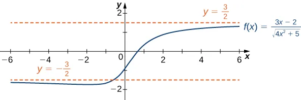
We conclude that limx→∞f(x)=−53, and the graph of f approaches the horizontal asymptote y=−53 as To find the limit as use the fact that as to conclude that and therefore the graph of approaches the horizontal asymptote as
Hint
limx→∞ex=∞ and limx→∞ex=0.
Answer
limx→∞f(x)=53,limx→-∞f(x)=−2
L,
y=L
∞
-∞,
f
f
f(x)=q(x)p(x),
f
f(x)=q(x)p(x)=g(x)+q(x)r(x),
where the degree of r(x) is less than the degree of q(x). The values of f(x) approach the values of g(x) as x→±∞. If g(x) is a linear function, it is known as an oblique asymptote.
Determine whether f has any vertical asymptotes.
Calculate f′. Find all critical points and determine the intervals where f is increasing and where f is decreasing. Determine whether f has any local extrema.
Calculate f′′. Determine the intervals where f is concave up and where f is concave down. Use this information to determine whether f has any inflection points. The second derivative can also be used as an alternate means to determine or verify that f has a local extremum at a critical point.
y
(0,2).
x
(x−1)2(x+2)=0,
x
(1,0)
(−2,0)
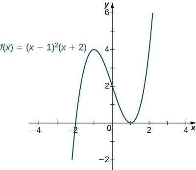
Step 3. We need to evaluate the end behavior of f. As x→∞,(x−1)2→∞ and (x+2)→∞. Therefore, limx→∞f(x)=∞. As x→-∞,(x−1)2→∞ and (x+2)→-∞. Therefore, limx→-∞f(x)=-∞. To get even more information about the end behavior of f, we can multiply the factors of f. When doing so, we see that
f(x)=(x−1)2(x+2)=x3−3x+2.
Since the leading term of f is x3, we conclude that f behaves like y=x3 as x→±∞.
Step 4. Since f is a polynomial function, it does not have any vertical asymptotes.
Step 5. The first derivative of f is
f′(x)=3x2−3.
Therefore, f has two critical points: x=1,−1. Divide the interval (-∞,∞) into the three smaller intervals: (-∞,−1),(−1,1), and (1,∞). Then, choose test points x=−2,x=0, and x=2 from these intervals and evaluate the sign of f′(x) at each of these test points, as shown in the following table.
Interval
Test Point
Sign of Derivative f′(x)=3x2−3=3(x−1)(x+1)
Conclusion
(-∞,−1)
x=−2
(+)(-)(-)=+
f is increasing.
(−1,1)
x=0
(+)(-)(+)=-
f is decreasing.
(1,∞)
x=2
(+)(+)(+)=+
f is increasing.
From the table, we see that f has a local maximum at x=−1 and a local minimum at x=1. Evaluating f(x) at those two points, we find that the local maximum value is f(−1)=4 and the local minimum value is f(1)=0.
Step 6. The second derivative of f is
f′′(x)=6x.
The second derivative is zero at x=0. Therefore, to determine the concavity of f, divide the interval (-∞,∞) into the smaller intervals (-∞,0) and (0,∞), and choose test points x=−1 and x=1 to determine the concavity of f on each of these smaller intervals as shown in the following table.
Interval
Test Point
Sign of f′′(x)=6x
Conclusion
(-∞,0)
x=−1
−
f is concave down.
(0,∞)
x=1
+
f is concave up.
We note that the information in the preceding table confirms the fact, found in step 5, that f has a local maximum at x=−1 and a local minimum at x=1. In addition, the information found in step 5—namely, f has a local maximum at x=−1 and a local minimum at x=1, and f′(x)=0 at those points—combined with the fact that f′′ changes sign only at x=0 confirms the results found in step 6 on the concavity of f.
Combining this information, we arrive at the graph of f(x)=(x−1)2(x+2) shown in the following graph.
Step 1. The function f is defined as long as the denominator is not zero. Therefore, the domain is the set of all real numbers x except x=±1.
Step 2. Find the intercepts. If x=0, then f(x)=0, so 0 is an intercept. If y=0, then (1−x2)x2=0, which implies x=0. Therefore, (0,0) is the only intercept.
Step 3. Evaluate the limits at infinity. Since f is a rational function, divide the numerator and denominator by the highest power in the denominator: x2. We obtain
x→±∞lim1−x2x2=x→±∞limx21−11=−1.
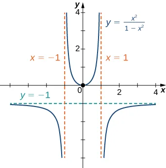
Therefore, f has a horizontal asymptote of y=−1 as x→∞ and x→-∞.
Step 4. To determine whether f has any vertical asymptotes, first check to see whether the denominator has any zeroes. We find the denominator is zero when x=±1. To determine whether the lines x=1 or x=−1 are vertical asymptotes of f, evaluate limx→1f(x) and limx→-1f(x). By looking at each one-sided limit as x→1, we see that
x→1+lim1−x2x2=-∞andx→1−lim1−x2x2=∞.
In addition, by looking at each one-sided limit as x→-1, we find that
x→-1+lim1−x2x2=∞andx→-1−lim1−x2x2=-∞.
Step 5. Calculate the first derivative:
f′(x)=(1−x2)2(1−x2)(2x)−x2(−2x)=(1−x2)22x.
Critical points occur at points x where f′(x)=0 or f′(x) is undefined. We see that f′(x)=0 when x=0. The derivative f′ is not undefined at any point in the domain of f. However, x=±1 are not in the domain of f. Therefore, to determine where f is increasing and where f is decreasing, divide the interval (-∞,∞) into four smaller intervals: (-∞,−1),(−1,0),(0,1), and (1,∞), and choose a test point in each interval to determine the sign of f′(x) in each of these intervals. The values x=−2,x=−21,x=21, and x=2 are good choices for test points as shown in the following table.
Interval
Test Point
Sign of f′(x)=(1−x2)22x
Conclusion
(-∞,−1)
x=−2
-/+=-
f is decreasing.
(−1,0)
x=−1/2
-/+=-
f is decreasing.
(0,1)
x=1/2
+/+=+
f is increasing.
(1,∞)
x=2
+/+=+
f is increasing.
From this analysis, we conclude that f has a local minimum at x=0 but no local maximum.
To determine the intervals where f is concave up and where f is concave down, we first need to find all points x where f′′(x)=0 or f′′(x) is undefined. Since the numerator 6x2+2=0 for any x,f′′(x) is never zero. Furthermore, f′′ is not undefined for any x in the domain of f. However, as discussed earlier, x=±1 are not in the domain of f. Therefore, to determine the concavity of f, we divide the interval (-∞,∞) into the three smaller intervals (-∞,−1),(−1,−1), and (1,∞), and choose a test point in each of these intervals to evaluate the sign of f′′(x). in each of these intervals. The values x=−2,x=0, and x=2 are possible test points as shown in the following table.
Interval
Test Point
Sign of f′′(x)=(1−x2)36x2+2
Conclusion
(-∞,−1)
x=−2
+/−=-
f is concave down.
(−1,−1)
x=0
+/+=+
f is concave up.
(1,∞)
x=2
+/−=-
f is concave down.
Combining all this information, we arrive at the graph of f shown below. Note that, although f changes concavity at x=−1 and x=1, there are no inflection points at either of these places because f is not continuous at x=−1 or x=1.
f
x→∞
x→-∞
f(x)
L.
x=a
f
x→a
∞
-∞.
Answer
x
x=1.
Step 2. Find the intercepts. We can see that when x=0,f(x)=0, so (0,0) is the only intercept.
Step 3. Evaluate the limits at infinity. Since the degree of the numerator is one more than the degree of the denominator, f must have an oblique asymptote. To find the oblique asymptote, use long division of polynomials to write
f(x)=x−1x2=x+1+x−11.
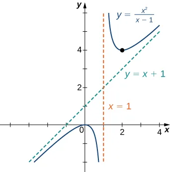
Since 1/(x−1)→0 as x→±∞,f(x) approaches the line y=x+1 as x→±∞. The line y=x+1 is an oblique asymptote for f.
Step 4. To check for vertical asymptotes, look at where the denominator is zero. Here the denominator is zero at x=1. Looking at both one-sided limits as x→1, we find
x→1+limx−1x2=∞andx→1−limx−1x2=-∞.
Therefore, x=1 is a vertical asymptote, and we have determined the behavior of f as x approaches 1 from the right and the left.
Step 5. Calculate the first derivative:
f′(x)=(x−1)2(x−1)(2x)−x2(1)=(x−1)2x2−2x.
We have f′(x)=0 when x2−2x=x(x−2)=0. Therefore, x=0 and x=2 are critical points. Since f is undefined at x=1, we need to divide the interval (-∞,∞) into the smaller intervals (-∞,0),(0,1),(1,2), and (2,∞), and choose a test point from each interval to evaluate the sign of f′(x) in each of these smaller intervals. For example, let x=−1,x=21,x=23, and x=3 be the test points as shown in the following table.
Interval
Test Point
Sign of f′(x)=(x−1)2x2−2x=(x−1)2x(x−2)
Conclusion
(-∞,0)
x=−1
(-)(-)/+=+
f is increasing.
(0,1)
x=1/2
(+)(-)/+=-
f is decreasing.
(1,2)
x=3/2
(+)(-)/+=-
f is decreasing.
(2,∞)
x=3
(+)(+)/+=+
f is increasing.
From this table, we see that f has a local maximum at x=0 and a local minimum at x=2. The value of f at the local maximum is f(0)=0 and the value of f at the local minimum is f(2)=4. Therefore, (0,0) and (2,4) are important points on the graph.
We see that f′′(x) is never zero or undefined for x in the domain of f. Since f is undefined at x=1, to check concavity we just divide the interval (-∞,∞) into the two smaller intervals (-∞,1) and (1,∞), and choose a test point from each interval to evaluate the sign of f′′(x) in each of these intervals. The values x=0 and x=2 are possible test points as shown in the following table.
Interval
Test Point
Sign of f′′(x)=(x−1)32
Conclusion
(-∞,1)
x=0
+/−=-
f is concave down.
(1,∞)
x=2
+/+=+
f is concave up.
From the information gathered, we arrive at the following graph for f.
Hint
Use long division of polynomials.
Answer
y=23x
f
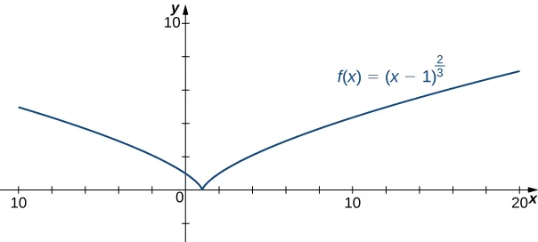
Step 2: To find the y-intercept, evaluate f(0). Since f(0)=1, the y-intercept is (0,1). To find the x-intercept, solve (x−1)2/3=0. The solution of this equation is x=1, so the x-intercept is (1,0).
Step 3: Since limx→±∞(x−1)2/3=∞, the function continues to grow without bound as x→∞ and x→-∞.
Step 4: The function has no vertical asymptotes.
Step 5: To determine where f is increasing or decreasing, calculate f′. We find
f′(x)=32(x−1)−1/3=3(x−1)1/32.
This function is not zero anywhere, but it is undefined when x=1. Therefore, the only critical point is x=1. Divide the interval (-∞,∞) into the smaller intervals (-∞,1) and (1,∞), and choose test points in each of these intervals to determine the sign of f′(x) in each of these smaller intervals. Let x=0 and x=2 be the test points as shown in the following table.
Interval
Test Point
Sign of f′(x)=3(x−1)1/32
Conclusion
(-∞,1)
x=0
+/−=-
f is decreasing.
(1,∞)
x=2
+/+=+
f is increasing.
We conclude that f has a local minimum at x=1. Evaluating f at x=1, we find that the value of f at the local minimum is zero. Note that f′(1) is undefined, so to determine the behavior of the function at this critical point, we need to examine limx→1f′(x). Looking at the one-sided limits, we have
x→1+lim3(x−1)1/32=∞andx→1−lim3(x−1)1/32=-∞.
Therefore, f has a cusp at x=1.
Step 6: To determine concavity, we calculate the second derivative of f:
f′′(x)=−92(x−1)−4/3=9(x−1)4/3−2.
We find that f′′(x) is defined for all x, but is undefined when x=1. Therefore, divide the interval (-∞,∞) into the smaller intervals (-∞,1) and (1,∞), and choose test points to evaluate the sign of f′′(x) in each of these intervals. As we did earlier, let x=0 and x=2 be test points as shown in the following table.
Interval
Test Point
Sign of f′′(x)=9(x−1)4/3−2
Conclusion
(-∞,1)
x=0
-/+=-
f is concave down.
(1,∞)
x=2
-/+=-
f is concave down.
From this table, we conclude that f is concave down everywhere. Combining all of this information, we arrive at the following graph for f.
f′(a)
x→a
f′(x)
+∞,
-∞.
Answer
The function f has a cusp at (0,5)limx→0−f′(x)=∞,limx→0+f′(x)=-∞. For end behavior, limx→±∞f(x)=-∞.
∞
x→∞
f(x)
x
f(x)
-∞
x→∞
f(x)<0
∣f(x)∣
x
f(x)
x
-∞
For a polynomial function p(x)=anxn+an−1xn−1+…+a1x+a0, where an=0, the end behavior is determined by the leading term anxn. If n=0,p(x) approaches ∞ or -∞ at each end.
For a rational function f(x)=q(x)p(x), the end behavior is determined by the relationship between the degree of p and the degree of q. If the degree of p is less than the degree of q, the line y=0 is a horizontal asymptote for f. If the degree of p is equal to the degree of q, then the line y=bnan is a horizontal asymptote, where an and bn are the leading coefficients of p and q, respectively. If the degree of p is greater than the degree of q, then f approaches ∞ or -∞ at each end.
x→±∞
for all x=0. Also, since
x→∞limx−1=0=x→∞limx1,
we can apply the squeeze theorem to conclude that
x→∞limxsinx=0.
Similarly,
x→-∞limxsinx=0.
Thus, f(x)=xsinx has a horizontal asymptote of y=0 and f(x) approaches this horizontal asymptote as x→±∞ as shown in the following graph.
(-π/2,π/2)
f(x)=tan−1(x)
limx→-∞2x4=∞.
Therefore f has a horizontal asymptote of y=0 as shown in the following graph.
As x→±∞, the denominator approaches 1. As x→∞, the numerator approaches +∞. As x→-∞, the numerator approaches -∞. Therefore limx→∞f(x)=∞, whereas limx→-∞f(x)=-∞ as shown in the following figure.