2.2 The Limit of a Function

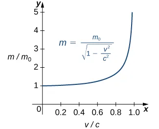
The concept of a limit or limiting process, essential to the understanding of calculus, has been around for thousands of years. In fact, early mathematicians used a limiting process to obtain better and better approximations of areas of circles. Yet, the formal definition of a limit—as we know and understand it today—did not appear until the late 19th century. We therefore begin our quest to understand limits, as our mathematical ancestors did, by using an intuitive approach. At the end of this chapter, armed with a conceptual understanding of limits, we examine the formal definition of a limit.

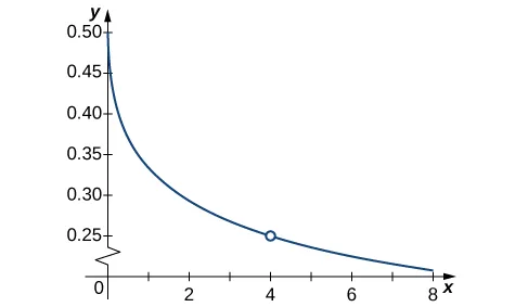
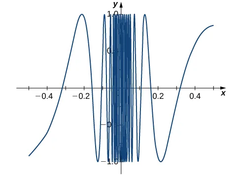
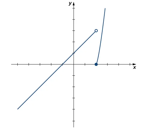
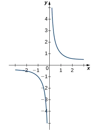
We begin our exploration of limits by taking a look at the graphs of the functions

f (x) = \frac{x ^{2} - 4}{x - 2}, g (x) = \frac{∣ x - 2∣}{x - 2}, and h (x) = \frac{1}{( x - 2 ) ^{2}},

which are shown in Figure 2.12. In particular, let’s focus our attention on the behavior of each graph at and around $x = 2.$

Three graphs of functions. The first is f(s) = (x^2 – 4) / (x-2), which is a line of slope, x intercept (-2,0), and open circle at (2,4). The second is g(x) = |x – 2 | / (x-2), which contains two lines: x=1 for x>2 and x= -1 for x < 2. There are open circles at both endpoints (2, 1) and (-2, 1). The third is h(x) = 1 / (x-2)^2, in which the function curves asymptotically towards y=0 and x=2 in quadrants one and two. — Figure 2.12These graphs show the behavior of three different functions around $x = 2.$

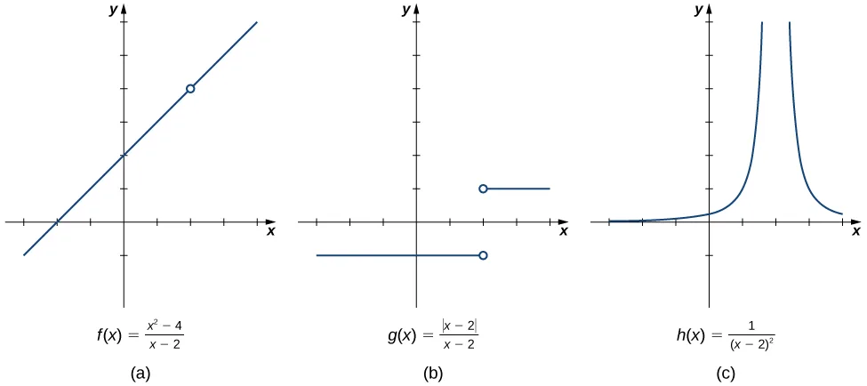
Each of the three functions is undefined at $x = 2,$ but if we make this statement and no other, we give a very incomplete picture of how each function behaves in the vicinity of $x = 2.$ To express the behavior of each graph in the vicinity of 2 more completely, we need to introduce the concept of a limit.

Intuitive Definition of a Limit

Let’s first take a closer look at how the function $f (x) = (x^{2} - 4) / (x - 2)$ behaves around $x = 2$ in Figure 2.12. As the values of x approach 2 from either side of 2, the values of $y = f (x)$ approach 4. Mathematically, we say that the limit of as approaches 2 is 4. Symbolically, we express this limit as

x \to 2 lim f (x) = 4.

From this very brief informal look at one limit, let’s start to develop an intuitive definition of the limit. We can think of the limit of a function at a number a as being the one real number L that the functional values approach as the x-values approach a, provided such a real number L exists. Stated more carefully, we have the following definition:

We can estimate limits by constructing tables of functional values and by looking at their graphs. This process is described in the following Problem-Solving Strategy.

Problem-Solving StrategyEvaluating a Limit Using a Table of Functional Values

To evaluate $lim_{x \to a} f (x),$ we begin by completing a table of functional values. We should choose two sets of x-values—one set of values approaching a and less than a, and another set of values approaching a and greater than a. Table 2.1 demonstrates what your tables might look like.
Next, let’s look at the values in each of the $f (x)$ columns and determine whether the values seem to be approaching a single value as we move down each column. In our columns, we look at the sequence $f (a - 0.1), f (a - 0.01), f (a - 0.001) ., f (a - 0.0001),$ and so on, and and so on. (: Although we have chosen the -values and so forth, and these values will probably work nearly every time, on very rare occasions we may need to modify our choices.)

We apply this Problem-Solving Strategy to compute a limit in Example 2.4.

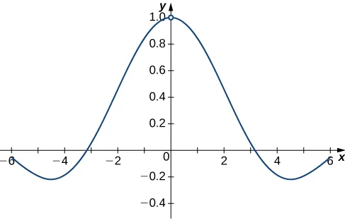
At this point, we see from Example 2.4 and Example 2.5 that it may be just as easy, if not easier, to estimate a limit of a function by inspecting its graph as it is to estimate the limit by using a table of functional values. In Example 2.6, we evaluate a limit exclusively by looking at a graph rather than by using a table of functional values.

Based on Example 2.6, we make the following observation: It is possible for the limit of a function to exist at a point, and for the function to be defined at this point, but the limit of the function and the value of the function at the point may be different.

Looking at a table of functional values or looking at the graph of a function provides us with useful insight into the value of the limit of a function at a given point. However, these techniques rely too much on guesswork. We eventually need to develop alternative methods of evaluating limits. These new methods are more algebraic in nature and we explore them in the next section; however, at this point we introduce two special limits that are foundational to the techniques to come.

We can make the following observations about these two limits.

For the first limit, observe that as x approaches a, so does $f (x),$ because $f (x) = x .$ Consequently, $lim_{x \to a} x = a .$
For the second limit, consider Table 2.4.

Table 2.4Table of Functional Values for

lim_{x \to a} c = c

f (x) = c

f (x) = c

Observe that for all values of x (regardless of whether they are approaching a), the values $f (x)$ remain constant at c. We have no choice but to conclude $lim_{x \to a} c = c .$

The Existence of a Limit

As we consider the limit in the next example, keep in mind that for the limit of a function to exist at a point, the functional values must approach a single real-number value at that point. If the functional values do not approach a single value, then the limit does not exist.

One-Sided Limits

Sometimes indicating that the limit of a function fails to exist at a point does not provide us with enough information about the behavior of the function at that particular point. To see this, we now revisit the function $g (x) = ∣ x - 2∣ / (x - 2)$ introduced at the beginning of the section (see Figure 2.12(b)). As we pick values of x close to 2, $g (x)$ does not approach a single value, so the limit as x approaches 2 does not exist—that is, $lim_{x \to 2} g (x)$ DNE. However, this statement alone does not give us a complete picture of the behavior of the function around the -value 2. To provide a more accurate description, we introduce the idea of a . For all values to the left of 2 (or 2), Thus, as approaches 2 from the left, approaches −1. Mathematically, we say that the limit as approaches 2 from the left is −1. Symbolically, we express this idea as

x \to 2^{-} lim g (x) = - 1.

Similarly, as x approaches 2 from the right (or from the positive side), $g (x)$ approaches 1. Symbolically, we express this idea as

x \to 2^{+} lim g (x) = 1.

We can now present an informal definition of one-sided limits.

Let us now consider the relationship between the limit of a function at a point and the limits from the right and left at that point. It seems clear that if the limit from the right and the limit from the left have a common value, then that common value is the limit of the function at that point. Similarly, if the limit from the left and the limit from the right take on different values, the limit of the function does not exist. These conclusions are summarized in Relating One-Sided and Two-Sided Limits.

Infinite Limits

Evaluating the limit of a function at a point or evaluating the limit of a function from the right and left at a point helps us to characterize the behavior of a function around a given value. As we shall see, we can also describe the behavior of functions that do not have finite limits.

We now turn our attention to $h (x) = 1 / (x - 2)^{2},$ the third and final function introduced at the beginning of this section (see Figure 2.12(c)). From its graph we see that as the values of x approach 2, the values of $h (x) = 1 / (x - 2)^{2}$ become larger and larger and, in fact, become infinite. Mathematically, we say that the limit of $h (x)$ as approaches 2 is positive infinity. Symbolically, we express this idea as

x \to 2 lim h (x) = + \infty.

More generally, we define infinite limits as follows:

It is important to understand that when we write statements such as $lim_{x \to a} f (x) = + \infty$ or $lim_{x \to a} f (x) = - \infty$ we are describing the behavior of the function, as we have just defined it. We are not asserting that a limit exists. For the limit of a function $f (x)$ to exist at , it must approach a real number as approaches . That said, if, for example, we always write rather than DNE.

It is useful to point out that functions of the form $f (x) = 1 / (x - a)^{n},$ where n is a positive integer, have infinite limits as x approaches a from either the left or right (Figure 2.20). These limits are summarized in Infinite Limits from Positive Integers.

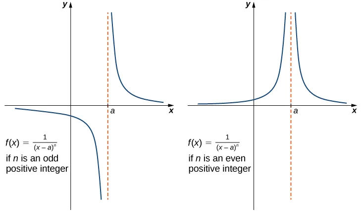
Two graphs side by side of f(x) = 1 / (x-a)^n. The first graph shows the case where n is an odd positive integer, and the second shows the case where n is an even positive integer. In the first, the graph has two segments. Each curve asymptotically towards the x axis, also known as y=0, and x=a. The segment to the left of x=a is below the x axis, and the segment to the right of x=a is above the x axis. In the second graph, both segments are above the x axis. — Figure 2.20The function $f (x) = 1 / (x - a)^{n}$ has infinite limits at a.

We should also point out that in the graphs of $f (x) = 1 / (x - a)^{n},$ points on the graph having x-coordinates very near to a are very close to the vertical line $x = a .$ That is, as x approaches a, the points on the graph of $f (x)$ are closer to the line $x = a .$ The line is called a of the graph. We formally define a vertical asymptote as follows:

In the next example we put our knowledge of various types of limits to use to analyze the behavior of a function at several different points.

Key Concepts

A table of values or graph may be used to estimate a limit.
If the limit of a function at a point does not exist, it is still possible that the limits from the left and right at that point may exist.
If the limits of a function from the left and right exist and are equal, then the limit of the function is that common value.
We may use limits to describe infinite behavior of a function at a point.

Key Equations

Intuitive Definition of the Limit	$lim_{x \to a} f (x) = L$
Two Important Limits	$lim_{x \to a} x = a lim_{x \to a} c = c$