2.3 The Limit Laws

In the previous section, we evaluated limits by looking at graphs or by constructing a table of values. In this section, we establish laws for calculating limits and learn how to apply these laws. In the Student Project at the end of this section, you have the opportunity to apply these limit laws to derive the formula for the area of a circle by adapting a method devised by the Greek mathematician Archimedes. We begin by restating two useful limit results from the previous section. These two results, together with the limit laws, serve as a foundation for calculating many limits.

Evaluating Limits with the Limit Laws

The first two limit laws were stated in Two Important Limits and we repeat them here. These basic results, together with the other limit laws, allow us to evaluate limits of many algebraic functions.

We now take a look at the limit laws, the individual properties of limits. The proofs that these laws hold are omitted here.

We now practice applying these limit laws to evaluate a limit.

Limits of Polynomial and Rational Functions

By now you have probably noticed that, in each of the previous examples, it has been the case that $lim_{x \to a} f (x) = f (a) .$ This is not always true, but it does hold for all polynomials for any choice of a and for all rational functions at all values of a for which the rational function is defined.

To see that this theorem holds, consider the polynomial $p (x) = c_{n} x^{n} + c_{n - 1} x^{n - 1} + \dots + c_{1} x + c_{0} .$ By applying the sum, constant multiple, and power laws, we end up with

lim_{x \to a} p (x) = lim_{x \to a} (c_{n} x^{n} + c_{n - 1} x^{n - 1} + \dots + c_{1} x + c_{0}) = c_{n} (lim_{x \to a} x)^{n} + c_{n - 1} (lim_{x \to a} x)^{n - 1} + \dots + c_{1} (lim_{x \to a} x) + lim_{x \to a} c_{0} = c_{n} a^{n} + c_{n - 1} a^{n - 1} + \dots + c_{1} a + c_{0} = p (a) .

It now follows from the quotient law that if $p (x)$ and $q (x)$ are polynomials for which $q (a) \neq = 0,$ then

x \to a lim \frac{p ( x )}{q ( x )} = \frac{p ( a )}{q ( a )} .

Example 2.16 applies this result.

Additional Limit Evaluation Techniques

As we have seen, we may evaluate easily the limits of polynomials and limits of some (but not all) rational functions by direct substitution. However, as we saw in the introductory section on limits, it is certainly possible for $lim_{x \to a} f (x)$ to exist when $f (a)$ is undefined. The following observation allows us to evaluate many limits of this type:

If for all $x \neq = a, f (x) = g (x)$ over some open interval containing a, then $lim_{x \to a} f (x) = lim_{x \to a} g (x) .$

To understand this idea better, consider the limit $lim_{x \to 1} \frac{x ^{2} - 1}{x - 1} .$

The function

f (x) = \frac{x ^{2} - 1}{x - 1} = \frac{( x - 1 ) ( x + 1 )}{x - 1}

and the function $g (x) = x + 1$ are identical for all values of $x \neq = 1.$ The graphs of these two functions are shown in Figure 2.24.

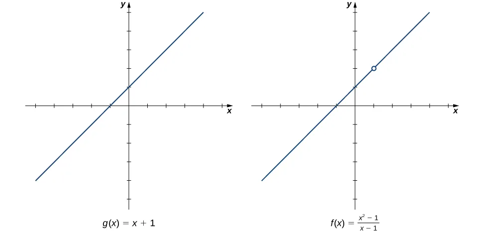
Two graphs side by side. The first is a graph of g(x) = x + 1, a linear function with y intercept at (0,1) and x intercept at (-1,0). The second is a graph of f(x) = (x^2 – 1) / (x – 1). This graph is identical to the first for all x not equal to 1, as there is an open circle at (1,2) in the second graph. — Figure 2.24The graphs of $f (x)$ and $g (x)$ are identical for all $x \neq = 1.$ Their limits at 1 are equal.

We see that

lim_{x \to 1} \frac{x ^{2} - 1}{x - 1} = lim_{x \to 1} \frac{( x - 1 ) ( x + 1 )}{x - 1} = lim_{x \to 1} (x + 1) = 2.

The limit has the form $lim_{x \to a} \frac{f ( x )}{g ( x )},$ where $lim_{x \to a} f (x) = 0$ and (In this case, we say that has the indeterminate form The following Problem-Solving Strategy provides a general outline for evaluating limits of this type.

The next examples demonstrate the use of this Problem-Solving Strategy. Example 2.17 illustrates the factor-and-cancel technique; Example 2.18 shows multiplying by a conjugate. In Example 2.19, we look at simplifying a complex fraction.

Example 2.20 does not fall neatly into any of the patterns established in the previous examples. However, with a little creativity, we can still use these same techniques.

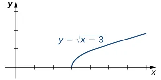
Let’s now revisit one-sided limits. Simple modifications in the limit laws allow us to apply them to one-sided limits. For example, to apply the limit laws to a limit of the form $lim_{x \to a^{-}} h (x),$ we require the function $h (x)$ to be defined over an open interval of the form $(b, a);$ for a limit of the form $lim_{x \to a^{+}} h (x),$ we require the function to be defined over an open interval of the form Example 2.21 illustrates this point.

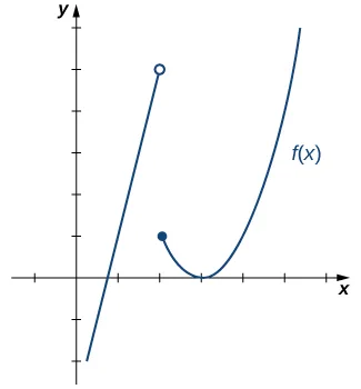
In Example 2.22 we look at one-sided limits of a piecewise-defined function and use these limits to draw a conclusion about a two-sided limit of the same function.

We now turn our attention to evaluating a limit of the form $lim_{x \to a} \frac{f ( x )}{g ( x )},$ where $lim_{x \to a} f (x) = K,$ where and That is, has the form at .

The Squeeze Theorem

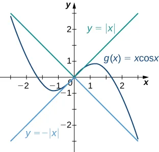
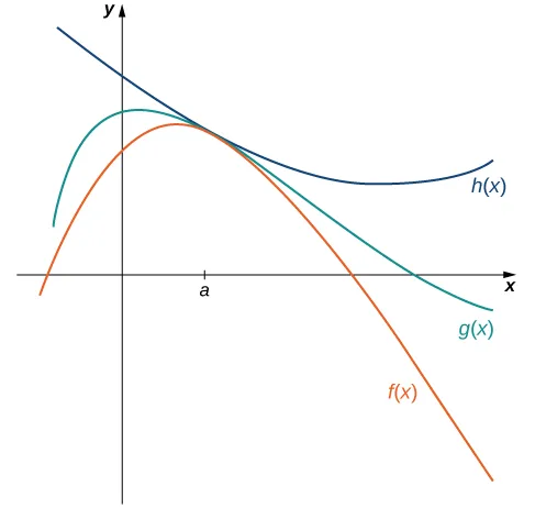
The techniques we have developed thus far work very well for algebraic functions, but we are still unable to evaluate limits of very basic trigonometric functions. The next theorem, called the squeeze theorem, proves very useful for establishing basic trigonometric limits. This theorem allows us to calculate limits by “squeezing” a function, with a limit at a point a that is unknown, between two functions having a common known limit at a. Figure 2.27 illustrates this idea.

A graph of three functions over a small interval. All three functions curve. Over this interval, the function g(x) is trapped between the functions h(x), which gives greater y values for the same x values, and f(x), which gives smaller y values for the same x values. The functions all approach the same limit when x=a. — Figure 2.27The Squeeze Theorem applies when $f (x) \leq g (x) \leq h (x)$ and $lim_{x \to a} f (x) = lim_{x \to a} h (x) .$

We now use the squeeze theorem to tackle several very important limits. Although this discussion is somewhat lengthy, these limits prove invaluable for the development of the material in both the next section and the next chapter. The first of these limits is $lim_{θ \to 0} sin θ .$ Consider the unit circle shown in Figure 2.29. In the figure, we see that $sin θ$ is the y-coordinate on the unit circle and it corresponds to the line segment shown in blue. The radian measure of angle θ is the length of the arc it subtends on the unit circle. Therefore, we see that for $0 < θ < \frac{π}{2}, 0 < sin θ < θ .$

A diagram of the unit circle in the x,y plane – it is a circle with radius 1 and center at the origin. A specific point (cos(theta), sin(theta)) is labeled in quadrant 1 on the edge of the circle. This point is one vertex of a right triangle inside the circle, with other vertices at the origin and (cos(theta), 0). As such, the lengths of the sides are cos(theta) for the base and sin(theta) for the height, where theta is the angle created by the hypotenuse and base. The radian measure of angle theta is the length of the arc it subtends on the unit circle. The diagram shows that for 0 < theta < pi/2, 0 < sin(theta) < theta. — Figure 2.29The sine function is shown as a line on the unit circle.

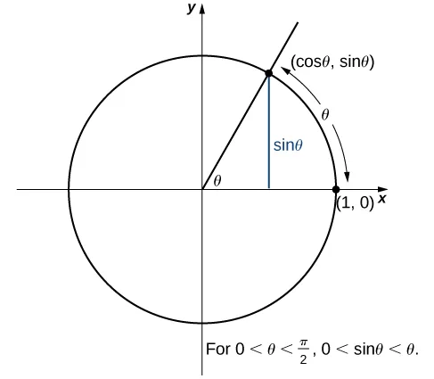
Because $lim_{θ \to 0^{+}} 0 = 0$ and $lim_{θ \to 0^{+}} θ = 0,$ by using the squeeze theorem we conclude that

θ \to 0^{+} lim sin θ = 0.

To see that $lim_{θ \to 0^{-}} sin θ = 0$ as well, observe that for $- \frac{π}{2} < θ < 0, 0 < - θ < \frac{π}{2}$ and hence, Consequently, It follows that An application of the squeeze theorem produces the desired limit. Thus, since and

θ \to 0 lim sin θ = 0.

Next, using the identity $cos θ = 1 - sin^{2} θ$ for $- \frac{π}{2} < θ < \frac{π}{2},$ we see that

θ \to 0 lim cos θ = θ \to 0 lim 1 - sin^{2} θ = 1.

We now take a look at a limit that plays an important role in later chapters—namely, $lim_{θ \to 0} \frac{s i n θ}{θ} .$ To evaluate this limit, we use the unit circle in Figure 2.30. Notice that this figure adds one additional triangle to Figure 2.30. We see that the length of the side opposite angle θ in this new triangle is $tan θ .$ Thus, we see that for $0 < θ < \frac{π}{2}, sin θ < θ < tan θ .$

The same diagram as the previous one. However, the triangle is expanded. The base is now from the origin to (1,0). The height goes from (1,0) to (1, tan(theta)). The hypotenuse goes from the origin to (1, tan(theta)). As such, the height is now tan(theta). It shows that for 0 < theta < pi/2, sin(theta) < theta < tan(theta). — Figure 2.30The sine and tangent functions are shown as lines on the unit circle.

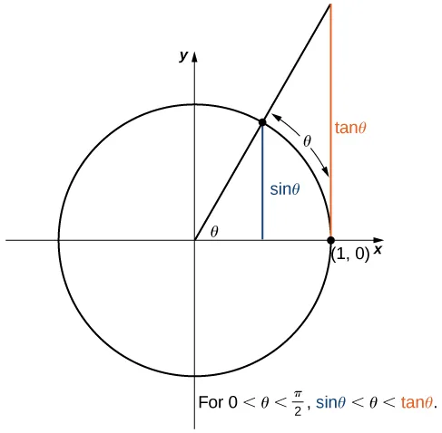
By dividing by $sin θ$ in all parts of the inequality, we obtain

1 < \frac{θ}{sin θ} < \frac{1}{cos θ} .

Equivalently, we have

1 > \frac{sin θ}{θ} > cos θ .

Since $lim_{θ \to 0^{+}} 1 = 1 = lim_{θ \to 0^{+}} cos θ,$ we conclude that By applying a manipulation similar to that used in demonstrating that we can show that Thus,

θ \to 0 lim \frac{sin θ}{θ} = 1.

In Example 2.25 we use this limit to establish $lim_{θ \to 0} \frac{1 - c o s θ}{θ} = 0.$ This limit also proves useful in later chapters.

Student ProjectDeriving the Formula for the Area of a Circle

Some of the geometric formulas we take for granted today were first derived by methods that anticipate some of the methods of calculus. The Greek mathematician Archimedes (ca. 287−212; BCE) was particularly inventive, using polygons inscribed within circles to approximate the area of the circle as the number of sides of the polygon increased. He never came up with the idea of a limit, but we can use this idea to see what his geometric constructions could have predicted about the limit.

We can estimate the area of a circle by computing the area of an inscribed regular polygon. Think of the regular polygon as being made up of n triangles. By taking the limit as the vertex angle of these triangles goes to zero, you can obtain the area of the circle. To see this, carry out the following steps:

Express the height h and the base b of the isosceles triangle in Figure 2.31 in terms of $θ$ and r.
Using the expressions that you obtained in step 1, express the area of the isosceles triangle in terms of θ and r.
(Substitute $(1 / 2) sin θ$ for $sin (θ / 2) cos (θ / 2)$ in your expression.)

Key Concepts

The limit laws allow us to evaluate limits of functions without having to go through step-by-step processes each time.
For polynomials and rational functions, $lim_{x \to a} f (x) = f (a) .$
You can evaluate the limit of a function by factoring and canceling, by multiplying by a conjugate, or by simplifying a complex fraction.
The squeeze theorem allows you to find the limit of a function if the function is always greater than one function and less than another function with limits that are known.

Key Equations

Basic Limit Results	$lim_{x \to a} x = a lim_{x \to a} c = c$
Important Limits	$lim_{θ \to 0} sin θ = 0$