2.4 Continuity

Many functions have the property that their graphs can be traced with a pencil without lifting the pencil from the page. Such functions are called continuous. Other functions have points at which a break in the graph occurs, but satisfy this property over intervals contained in their domains. They are continuous on these intervals and are said to have a discontinuity at a point where a break occurs.

We begin our investigation of continuity by exploring what it means for a function to have continuity at a point. Intuitively, a function is continuous at a particular point if there is no break in its graph at that point.

Continuity at a Point

Before we look at a formal definition of what it means for a function to be continuous at a point, let’s consider various functions that fail to meet our intuitive notion of what it means to be continuous at a point. We then create a list of conditions that prevent such failures.

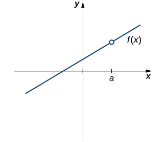
Our first function of interest is shown in Figure 2.32. We see that the graph of $f(x)$ has a hole at a. In fact, $f(a)$ is undefined. At the very least, for $f(x)$ to be continuous at a, we need the following condition:

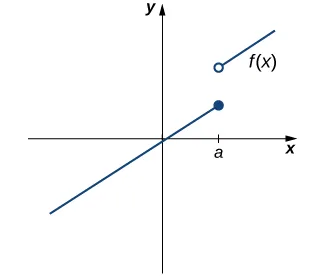
However, as we see in Figure 2.33, this condition alone is insufficient to guarantee continuity at the point a. Although $f(a)$ is defined, the function has a gap at a. In this example, the gap exists because ${\lim }_{x\to a}f(x)$ does not exist. We must add another condition for continuity at a—namely,

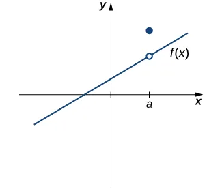
However, as we see in Figure 2.34, these two conditions by themselves do not guarantee continuity at a point. The function in this figure satisfies both of our first two conditions, but is still not continuous at a. We must add a third condition to our list:

Now we put our list of conditions together and form a definition of continuity at a point.

The following procedure can be used to analyze the continuity of a function at a point using this definition.

The next three examples demonstrate how to apply this definition to determine whether a function is continuous at a given point. These examples illustrate situations in which each of the conditions for continuity in the definition succeed or fail.

By applying the definition of continuity and previously established theorems concerning the evaluation of limits, we can state the following theorem.

Proof

Previously, we showed that if $p(x)$ and $q(x)$ are polynomials, ${\lim }_{x\to a}p(x)=p(a)$ for every polynomial $p(x)$ and ${\lim }_{x\to a}\frac{p(x)}{q(x)}=\frac{p(a)}{q(a)}$ as long as $q(a)\ne 0.$ Therefore, polynomials and rational functions are continuous on their domains.

□

We now apply Continuity of Polynomials and Rational Functions to determine the points at which a given rational function is continuous.

Types of Discontinuities

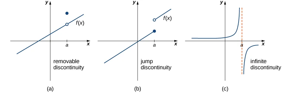
As we have seen in Example 2.26 and Example 2.27, discontinuities take on several different appearances. We classify the types of discontinuities we have seen thus far as removable discontinuities, infinite discontinuities, or jump discontinuities. Intuitively, a removable discontinuity is a discontinuity for which there is a hole in the graph, a jump discontinuity is a noninfinite discontinuity for which the sections of the function do not meet up, and an infinite discontinuity is a discontinuity located at a vertical asymptote. Figure 2.37 illustrates the differences in these types of discontinuities. Although these terms provide a handy way of describing three common types of discontinuities, keep in mind that not all discontinuities fit neatly into these categories.

These three discontinuities are formally defined as follows:

Continuity over an Interval

Now that we have explored the concept of continuity at a point, we extend that idea to continuity over an interval. As we develop this idea for different types of intervals, it may be useful to keep in mind the intuitive idea that a function is continuous over an interval if we can use a pencil to trace the function between any two points in the interval without lifting the pencil from the paper. In preparation for defining continuity on an interval, we begin by looking at the definition of what it means for a function to be continuous from the right at a point and continuous from the left at a point.

A function is continuous over an open interval if it is continuous at every point in the interval. A function $f(x)$ is continuous over a closed interval of the form $[a,b]$ if it is continuous at every point in $(a,b)$ and is continuous from the right at a and is continuous from the left at b. Analogously, a function $f(x)$ is continuous over an interval of the form $(a,b]$ if it is continuous over $(a,b)$ and is continuous from the left at b. Continuity over other types of intervals are defined in a similar fashion.

Requiring that ${\lim }_{x\to a^{+}}f(x)=f(a)$ and ${\lim }_{x\to b^{-}}f(x)=f(b)$ ensures that we can trace the graph of the function from the point $(a,f(a))$ to the point $(b,f(b))$ without lifting the pencil. If, for example, ${\lim }_{x\to a^{+}}f(x)\ne f(a),$ we would need to lift our pencil to jump from $f(a)$ to the graph of the rest of the function over $(a,b].$

The Composite Function Theorem allows us to expand our ability to compute limits. In particular, this theorem ultimately allows us to demonstrate that trigonometric functions are continuous over their domains.

Before we move on to Example 2.35, recall that earlier, in the section on limit laws, we showed ${\lim }_{x\to 0}\cos x=1=\cos (0).$ Consequently, we know that $f(x)=\cos x$ is continuous at 0. In Example 2.35 we see how to combine this result with the composite function theorem.

The proof of the next theorem uses the composite function theorem as well as the continuity of $f(x)=\sin x$ and $g(x)=\cos x$ at the point 0 to show that trigonometric functions are continuous over their entire domains.

Proof

We begin by demonstrating that $\cos x$ is continuous at every real number. To do this, we must show that ${\lim }_{x\to a}\cos x=\cos a$ for all values of a.

$\begin{array}{lllll}{\lim }_{x\to a}\cos x& ={\lim }_{x\to a}\cos ((x-a)+a)& & & \text{rewrite}x=x-a+a\\ & ={\lim }_{x\to a}(\cos (x-a)\cos a-\sin (x-a)\sin a)& & & \text{apply the identity for the cosine of the sum of two angles}\\ & =\cos ({\lim }_{x\to a}(x-a))\cos a-\sin ({\lim }_{x\to a}(x-a))\sin a& & & {\lim }_{x\to a}(x-a)=0,\text{and}\sin x\text{and}\cos x\text{are continuous at 0}\\ & =\cos (0)\cos a-\sin (0)\sin a& & & \text{evaluate cos(0) and sin(0) and simplify}\\ & =1\cdot \cos a-0\cdot \sin a=\cos a.& & & \end{array}$

The proof that $\sin x$ is continuous at every real number is analogous. Because the remaining trigonometric functions may be expressed in terms of $\sin x$ and $\cos x,$ their continuity follows from the quotient limit law.

□

As you can see, the composite function theorem is invaluable in demonstrating the continuity of trigonometric functions. As we continue our study of calculus, we revisit this theorem many times.

The Intermediate Value Theorem

Functions that are continuous over intervals of the form $[a,b],$ where a and b are real numbers, exhibit many useful properties. Throughout our study of calculus, we will encounter many powerful theorems concerning such functions. The first of these theorems is the Intermediate Value Theorem.

Key Concepts

• For a function to be continuous at a point, it must be defined at that point, its limit must exist at the point, and the value of the function at that point must equal the value of the limit at that point.
• Discontinuities may be classified as removable, jump, or infinite.
• A function is continuous over an open interval if it is continuous at every point in the interval. It is continuous over a closed interval if it is continuous at every point in its interior and is continuous at its endpoints.
• The composite function theorem states: If $f(x)$ is continuous at L and ${\lim }_{x\to a}g(x)=L,$ then ${\lim }_{x\to a}f(g(x))=f({\lim }_{x\to a}g(x))=f(L).$
• The Intermediate Value Theorem guarantees that if a function is continuous over a closed interval, then the function takes on every value between the values at its endpoints.