Having covered the essential concepts of chemical equilibria in the preceding sections of this chapter, this final section will demonstrate the more practical aspect of using these concepts and appropriate mathematical strategies to perform various equilibrium calculations. These types of computations are essential to many areas of science and technology—for example, in the formulation and dosing of pharmaceutical products. After a drug is ingested or injected, it is typically involved in several chemical equilibria that affect its ultimate concentration in the body system of interest. Knowledge of the quantitative aspects of these equilibria is required to compute a dosage amount that will solicit the desired therapeutic effect.
Many of the useful equilibrium calculations that will be demonstrated here require terms representing changes in reactant and product concentrations. These terms are derived from the stoichiometry of the reaction, as illustrated by decomposition of ammonia:
As shown earlier in this chapter, this equilibrium may be established within a sealed container that initially contains either NH₃ only, or a mixture of any two of the three chemical species involved in the equilibrium. Regardless of its initial composition, a reaction mixture will show the same relationships between changes in the concentrations of the three species involved, as dictated by the reaction stoichiometry (see also the related content on expressing reaction rates in the chapter on kinetics). For example, if the nitrogen concentration increases by an amount x:
the corresponding changes in the other species concentrations are
where the negative sign indicates a decrease in concentration.
Calculation of an Equilibrium Constant
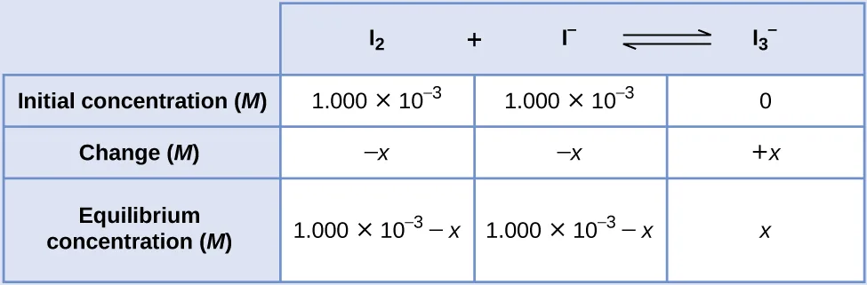
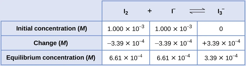
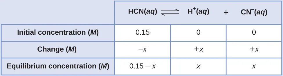
The equilibrium constant for a reaction is calculated from the equilibrium concentrations (or pressures) of its reactants and products. If these concentrations are known, the calculation simply involves their substitution into the K expression, as was illustrated by Example 13.2. A slightly more challenging example is provided next, in which the reaction stoichiometry is used to derive equilibrium concentrations from the information provided. The basic strategy of this computation is helpful for many types of equilibrium computations and relies on the use of terms for the reactant and product concentrations initially present, for how they change as the reaction proceeds, and for what they are when the system reaches equilibrium. The acronym ICE is commonly used to refer to this mathematical approach, and the concentrations terms are usually gathered in a tabular format called an ICE table.
Calculation of a Missing Equilibrium Concentration
When the equilibrium constant and all but one equilibrium concentration are provided, the other equilibrium concentration(s) may be calculated. A computation of this sort is illustrated in the next example exercise.
Calculation of Equilibrium Concentrations from Initial Concentrations
Perhaps the most challenging type of equilibrium calculation can be one in which equilibrium concentrations are derived from initial concentrations and an equilibrium constant. For these calculations, a four-step approach is typically useful:
- Identify the direction in which the reaction will proceed to reach equilibrium.
- Develop an ICE table.
- Calculate the concentration changes and, subsequently, the equilibrium concentrations.
- Confirm the calculated equilibrium concentrations.
The last two example exercises of this chapter demonstrate the application of this strategy.
Key Concepts and Summary
Calculating values for equilibrium constants and/or equilibrium concentrations is of practical benefit to many applications. A mathematical strategy that uses initial concentrations, changes in concentrations, and equilibrium concentrations (and goes by the acronym ICE) is useful for several types of equilibrium calculations.