13.2 Equilibrium Constants

The status of a reversible reaction is conveniently assessed by evaluating its reaction quotient (Q). For a reversible reaction described by

m A + n B ⇌ x C + y D

the reaction quotient is derived directly from the stoichiometry of the balanced equation as

Q_{c} = \frac{[ C ] ^{x} [ D ] ^{y}}{[ A ] ^{m} [ B ] ^{n}}

where the subscript c denotes the use of molar concentrations in the expression. If the reactants and products are gaseous, a reaction quotient may be similarly derived using partial pressures:

Q_{p} = \frac{P _{C} ^{x} P _{D} ^{y}}{P _{A} ^{m} P _{B} ^{n}}

Note that the reaction quotient equations above are a simplification of more rigorous expressions that use relative values for concentrations and pressures rather than absolute values. These relative concentration and pressure values are dimensionless (they have no units); consequently, so are the reaction quotients. For purposes of this introductory text, it will suffice to use the simplified equations and to disregard units when computing Q. In most cases, this will introduce only modest errors in calculations involving reaction quotients.

Four graphs are shown and labeled, “a,” “b,” “c,” and “d.” All four graphs have a vertical dotted line running through the middle labeled, “Equilibrium is reached.” The y-axis on graph a is labeled, “Concentration,” and the x-axis is labeled, “Time.” Three curves are plotted on graph a. The first is labeled, “[ S O subscript 2 ];” this line starts high on the y-axis, ends midway down the y-axis, has a steep initial slope and a more gradual slope as it approaches the far right on the x-axis. The second curve on this graph is labeled, “[ O subscript 2 ];” this line mimics the first except that it starts and ends about fifty percent lower on the y-axis. The third curve is the inverse of the first in shape and is labeled, “[ S O subscript 3 ].” The y-axis on graph b is labeled, “Concentration,” and the x-axis is labeled, “Time.” Three curves are plotted on graph b. The first is labeled, “[ S O subscript 2 ];” this line starts low on the y-axis, ends midway up the y-axis, has a steep initial slope and a more gradual slope as it approaches the far right on the x-axis. The second curve on this graph is labeled, “[ O subscript 2 ];” this line mimics the first except that it ends about fifty percent lower on the y-axis. The third curve is the inverse of the first in shape and is labeled, “[ S O subscript 3 ].” The y-axis on graph c is labeled, “Reaction Quotient,” and the x-axis is labeled, “Time.” A single curve is plotted on graph c. This curve begins at the bottom of the y-axis and rises steeply up near the top of the y-axis, then levels off into a horizontal line. The top point of this line is labeled, “k.” The y-axis on graph d is labeled, “Reaction Quotient,” and the x-axis is labeled, “Time.” A single curve is plotted on graph d. This curve begins near the edge of the top of the y-axis and falls steeply toward the x-axis, then levels off into a horizontal line. The bottom point of this line is labeled, “k.” — Figure 13.5Changes in concentrations and *Q $_{c}$* for a chemical equilibrium achieved beginning with (a) a mixture of reactants only and (b) products only.

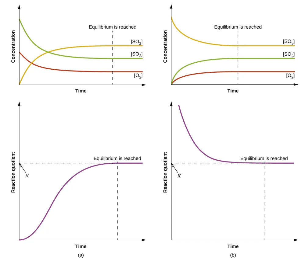
The numerical value of Q varies as a reaction proceeds towards equilibrium; therefore, it can serve as a useful indicator of the reaction’s status. To illustrate this point, consider the oxidation of sulfur dioxide:

2SO_{2} (g) + O_{2} (g) ⇌ 2SO_{3} (g)

Two different experimental scenarios are depicted in Figure 13.5, one in which this reaction is initiated with a mixture of reactants only, SO₂ and O₂, and another that begins with only product, SO₃. For the reaction that begins with a mixture of reactants only, Q is initially equal to zero:

Q_{c} = \frac{[ SO _{3} ] ^{2}}{[ SO _{2} ] ^{2} [ O _{2} ]} = \frac{0 ^{2}}{[ SO _{2} ] ^{2} [ O _{2} ]} = 0

As the reaction proceeds toward equilibrium in the forward direction, reactant concentrations decrease (as does the denominator of Q $_{c}$ ), product concentration increases (as does the numerator of Q $_{c}$ ), and the reaction quotient consequently increases. When equilibrium is achieved, the concentrations of reactants and product remain constant, as does the value of Q $_{c}$ .

If the reaction begins with only product present, the value of Q $_{c}$ is initially undefined (immeasurably large, or infinite):

Q_{c} = \frac{[ SO _{3} ] ^{2}}{[ SO _{2} ] ^{2} [ O _{2} ]} = \frac{[ SO _{3} ] ^{2}}{0} \to \infty

In this case, the reaction proceeds toward equilibrium in the reverse direction. The product concentration and the numerator of Q $_{c}$ decrease with time, the reactant concentrations and the denominator of Q $_{c}$ increase, and the reaction quotient consequently decreases until it becomes constant at equilibrium.

The constant value of Q exhibited by a system at equilibrium is called the equilibrium constant, K:

K \equiv Q at equilibrium

Comparison of the data plots in Figure 13.5 shows that both experimental scenarios resulted in the same value for the equilibrium constant. This is a general observation for all equilibrium systems, known as the law of mass action: At a given temperature, the reaction quotient for a system at equilibrium is constant.

By its definition, the magnitude of an equilibrium constant explicitly reflects the composition of a reaction mixture at equilibrium, and it may be interpreted with regard to the extent of the forward reaction. A reaction exhibiting a large K will reach equilibrium when most of the reactant has been converted to product, whereas a small K indicates the reaction achieves equilibrium after very little reactant has been converted. It’s important to keep in mind that the magnitude of K does not indicate how rapidly or slowly equilibrium will be reached. Some equilibria are established so quickly as to be nearly instantaneous, and others so slowly that no perceptible change is observed over the course of days, years, or longer.

The equilibrium constant for a reaction can be used to predict the behavior of mixtures containing its reactants and/or products. As demonstrated by the sulfur dioxide oxidation process described above, a chemical reaction will proceed in whatever direction is necessary to achieve equilibrium. Comparing Q to K for an equilibrium system of interest allows prediction of what reaction (forward or reverse), if any, will occur.

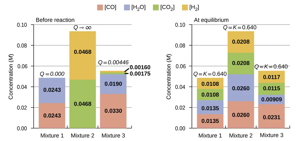
To further illustrate this important point, consider the reversible reaction shown below:

CO (g) + H_{2} O (g) ⇌ CO_{2} (g) + H_{2} (g) K_{c} = 0.640 T = 800 °C

The bar charts in Figure 13.6 represent changes in reactant and product concentrations for three different reaction mixtures. The reaction quotients for mixtures 1 and 3 are initially lesser than the reaction’s equilibrium constant, so each of these mixtures will experience a net forward reaction to achieve equilibrium. The reaction quotient for mixture 2 is initially greater than the equilibrium constant, so this mixture will proceed in the reverse direction until equilibrium is established.

Two sets of bar graphs are shown. The left is labeled, “Before reaction,” and the right is labeled, “At equilibrium.” Both graphs have y-axes labeled, “Concentration ( M ),” and three bars on the x-axes labeled, “Mixture 1,” “Mixture 2,” and “Mixture 3.” The y-axis has a scale beginning at 0.00 and ending at 0.10, with measurement increments of 0.02. The bars on the graphs are color coded and a key is provided with a legend. Red is labeled, “C O;” blue is labeled, “H subscript 2 O;” green is labeled, “C O subscript 2,” and yellow is labeled, “H subscript 2.” The graph on the left shows the red bar for mixture one just above 0.02, labeled “0.0243,” and the blue bar near 0.05, labeled “0.0243.” For mixture two, the green bar is near 0.05, labeled “0.0468,” and the yellow bar is near 0.09, labeled “0.0468.” For mixture 3, the red bar is near 0.01, labeled “0.0330,” the blue bar is slightly above that, labeled “0.190,” with green and yellow topping it off at 0.02. Green is labeled “0.00175” and yellow is labeled “0.00160.” On the right graph, the bar for mixture one shows the red bar slightly above 0.01, labeled “0.0135,” the blue bar stacked on it rising slightly above 0.02, labeled “0.0135,” the green rising near 0.04, labeled “0.0108,” and the yellow bar reaching near 0.05, labeled “0.0108.” A label above this bar reads, “Q equals 0.640.” The bar for mixture two shows the red bar slightly above 0.02, labeled “0.0260,” the blue bar stacked on it rising near 0.05, labeled “0.0260,” the green rising near 0.07, labeled “0.0208,” and the yellow bar reaching near 0.10, labeled “0.0208.” A label above this bar reads “Q equals 0.640.” The bar for mixture three shows the red bar near 0.01, labeled “0.0231,” the blue bar stacked on it rising slightly above 0.01, labeled “0.00909,” the green rising near 0.02, labeled “0.0115,” and the yellow bar reaching 0.02, labeled “0.0117.” A label above this bar reads “Q equals 0.640”. — Figure 13.6Compositions of three mixtures before (Q $_{c}$ ≠ K $_{c}$ ) and after (Q = K) equilibrium is established for the reaction

Homogeneous Equilibria

A homogeneous equilibrium is one in which all reactants and products (and any catalysts, if applicable) are present in the same phase. By this definition, homogeneous equilibria take place in solutions. These solutions are most commonly either liquid or gaseous phases, as shown by the examples below:

C_{2} H_{2} (a q) + 2 Br_{2} (a q) I_{2} (a q) + I^{-} (a q) HF (a q) + H_{2} O (l) NH_{3} (a q) + H_{2} O (l) ⇌ ⇌ ⇌ ⇌ C_{2} H_{2} Br_{4} (a q) I_{3}^{-} (a q) H_{3} O^{+} (a q) + F^{-} (a q) NH_{4}^{+} (a q) + OH^{-} (a q) K_{c} K_{c} K_{c} K_{c} = = = = \frac{[ C _{2} H _{2} Br _{4} ]}{[ C _{2} H _{2} ] [ Br _{2} ] ^{2}} \frac{[ I _{3} ^{-} ]}{[ I _{2} ] [ I ^{-} ]} \frac{[ H _{3} O ^{+} ] [ F ^{-} ]}{[ HF ]} \frac{[ NH _{4} ^{+} ] [ OH ^{-} ]}{[ NH _{3} ]}

These examples all involve aqueous solutions, those in which water functions as the solvent. In the last two examples, water also functions as a reactant, but its concentration is not included in the reaction quotient. The reason for this omission is related to the more rigorous form of the Q (or K) expression mentioned previously in this chapter, in which relative concentrations for liquids and solids are equal to 1 and needn’t be included. Consequently, reaction quotients include concentration or pressure terms only for gaseous and solute species.

The equilibria below all involve gas-phase solutions:

C_{2} H_{6} (g) 3 O_{2} (g) N_{2} (g) + 3 H_{2} (g) C_{3} H_{8} (g) + 5 O_{2} (g) ⇌ ⇌ ⇌ ⇌ C_{2} H_{4} (g) + H_{2} (g) 2 O_{3} (g) 2 NH_{3} (g) 3 CO_{2} (g) + 4 H_{2} O (g) K_{c} K_{c} K_{c} K_{c} = = = = \frac{[ C _{2} H _{4} ] [ H _{2} ]}{[ C _{2} H _{6} ]} \frac{[ O _{3} ] ^{2}}{[ O _{2} ] ^{3}} \frac{[ NH _{3} ] ^{2}}{[ N _{2} ] [ H _{2} ] ^{3}} \frac{[ CO _{2} ] ^{3} [ H _{2} O ] ^{4}}{[ C _{3} H _{8} ] [ O _{2} ] ^{5}}

For gas-phase solutions, the equilibrium constant may be expressed in terms of either the molar concentrations (K $_{c}$ ) or partial pressures (K $_{p}$ ) of the reactants and products. A relation between these two K values may be simply derived from the ideal gas equation and the definition of molarity:

P V = n R T

P = (\frac{n}{V}) R T

= M R T

where P is partial pressure, V is volume, n is molar amount, R is the gas constant, T is temperature, and M is molar concentration.

For the gas-phase reaction $a A + b B ⇌ c C + d D:$

K_{P} = \frac{( P _{C} ) ^{c} ( P _{D} ) ^{d}}{( P _{A} ) ^{a} ( P _{B} ) ^{b}}

= \frac{([ C] \times R T ) ^{c} ([ D] \times R T ) ^{d}}{([ A] \times R T ) ^{a} ([ B] \times R T ) ^{b}}

= \frac{[ C ] ^{c} [ D ] ^{d}}{[ A ] ^{a} [ B ] ^{b}} \times \frac{( R T ) ^{c + d}}{( R T ) ^{a + b}}

= K_{c} (R T)^{(c + d) - (a + b)}

= K_{c} (R T)^{Δ n}

And so, the relationship between K $_{c}$ and K $_{P}$ is

K_{P} = K_{c} (R T)^{Δ n}

where Δn is the difference in the molar amounts of product and reactant gases, in this case:

Δ n = (c + d) - (a + b)

Heterogeneous Equilibria

A heterogeneous equilibrium involves reactants and products in two or more different phases, as illustrated by the following examples:

PbCl_{2} (s) CaO (s) + CO_{2} (g) C (s) + 2 S (g) Br_{2} (l) ⇌ ⇌ ⇌ ⇌ Pb^{2 +} (a q) + 2 Cl^{-} (a q) CaCO_{3} (s) CS_{2} (g) Br_{2} (g) K_{c} K_{c} K_{c} K_{c} = = = = [Pb^{2 +}] [Cl^{-}]^{2} \frac{1}{[CO _{2} ]} \frac{[CS _{2} ]}{[ S ] ^{2}} [Br_{2} (g)]

Again, note that concentration terms are only included for gaseous and solute species, as discussed previously.

Two of the above examples include terms for gaseous species only in their equilibrium constants, and so K $_{p}$ expressions may also be written:

CaO (s) + CO_{2} (g) C (s) + 2 S (g) ⇌ ⇌ CaCO_{3} (s) CS_{2} (g) K_{P} K_{P} = = \frac{1}{P _{CO_{2}}} \frac{P _{CS_{2}}}{( P _{S} ) ^{2}}

Coupled Equilibria

The equilibrium systems discussed so far have all been relatively simple, involving just single reversible reactions. Many systems, however, involve two or more coupled equilibrium reactions, those which have in common one or more reactant or product species. Since the law of mass action allows for a straightforward derivation of equilibrium constant expressions from balanced chemical equations, the K value for a system involving coupled equilibria can be related to the K values of the individual reactions. Three basic manipulations are involved in this approach, as described below.

1. Changing the direction of a chemical equation essentially swaps the identities of “reactants” and “products,” and so the equilibrium constant for the reversed equation is simply the reciprocal of that for the forward equation.

A ⇌ B K_{c} = \frac{[ B ]}{[ A ]} B ⇌ A K_{c’} = \frac{[ A ]}{[ B ]}

K_{c’} = \frac{1}{K _{c}}

2. Changing the stoichiometric coefficients in an equation by some factor x results in an exponential change in the equilibrium constant by that same factor:

A ⇌ B K_{c} = \frac{[ B ]}{[ A ]} xA ⇌ xB K_{c’} = \frac{[ B ] ^{x}}{[ A ] ^{x}}

K_{c’} = K_{c}^{x}

3. Adding two or more equilibrium equations together yields an overall equation whose equilibrium constant is the mathematical product of the individual reaction’s K values:

A ⇌ B K_{c1} = \frac{[ B ]}{[ A ]} B ⇌ C K_{c2} = \frac{[ C ]}{[ B ]}

The net reaction for these coupled equilibria is obtained by summing the two equilibrium equations and canceling any redundancies:

A + B ⇌ B + C A + B ⇌ B + C A ⇌ C K_{c’} = \frac{[ C ]}{[ A ]}

Comparing the equilibrium constant for the net reaction to those for the two coupled equilibrium reactions reveals the following relationship:

K_{c1} K_{c2} = \frac{[ B ]}{[ A ]} \times \frac{[ C ]}{[ B ]} = \frac{[ B ] [ C ]}{[ A ] [ B ]} = \frac{[ C ]}{[ A ]} = K_{c’}

K_{c’} = K_{c1} K_{c2}

Example 13.5 demonstrates the use of this strategy in describing coupled equilibrium processes.

Key Concepts and Summary

The composition of a reaction mixture may be represented by a mathematical function known as the reaction quotient, Q. For a reaction at equilibrium, the composition is constant, and Q is called the equilibrium constant, K.

A homogeneous equilibrium is an equilibrium in which all components are in the same phase. A heterogeneous equilibrium is an equilibrium in which components are in two or more phases.

Key Equations

Q_{c} = \frac{[ C ] ^{x} [ D ] ^{y}}{[ A ] ^{m} [ B ] ^{n}} for the reaction m A + n B ⇌ x C + y D